Photosynthesis

Photosynthesis is a process which uses the energy of sunlight to convert carbon dioxide from the air into sugars. These sugars are subsequently transformed into other matter. They are the material and energetic basis of most organisms on earth, in particular of us humans. (Sure, there are some organisms living independently from sunlight. They are populating deep soil layers and the deep sea and they are more abundant than previously thought. This is not significant in terms of human nutrition, however. Our bodies – and the bodies of the organisms we are eating – are built 100% from sunlight and most of our bodies carbon comes from photosynthetic sugars.) In addition, photosynthesis is the process, which produces all the oxygen we are breathing, which has produced all those fossil fuels we are happily combusting and which eliminates all the carbon dioxide we are producing. (Well, unfortunately not precisely all of it.)

The following picture is meant to symbolize the process of photosynthesis. I leave it to your consideration, whether this has succeeded. (One clear shortcoming is the fact that it does not give any indication of the global importance of photosynthesis…)

Photosynthesis

Photosynthesis

Further reading:

Photosynthesis

Photosynthesis in the Deep?

Reinventing the leaf

Fine-tuning photosynthesis

Posted in Concepts | Tagged , , , , | Leave a comment

Root parasitizing nematodes

I have been working on root knot nematodes for a while, and here are some images featuring this interaction. The first image gives a summary, by and large, of nematodes damaging plant roots: First there are several kinds of free-living nematodes feeding directly on plant tissue (depicted here in blue color). Starting from this way of living, two major groups have evolved a sedentary life style. These are root knot nematodes, forming root galls and large gelatinous masses containing numerous eggs (see next image, upper left part) and root cyst nematodes, protecting their eggs in lemon-shaped cysts (next image, lower part).

Parasitic Nematodes

Parasitic Nematodes

Below I will focus on root knot nematodes and the following image gives a summary of their life cycle: Nematode eggs contain already fully functional juvenile nematodes, which hatch under suitable conditions. Within the eggs nematodes can survive long periods of adverse conditions in the soil. After hatching nematodes try to find a suitable root and to enter this root either at the root tip or at root branching sites. Inside the root nematodes establish galls (here shown within a transparent root), by inducing abnormal growth of plant cells. The nematodes then feed from the contents of these structures, finally producing large numbers of eggs, protected within a large gelatinous matrix (egg mass).

Overview root knot nematodes

Overview root knot nematodes

The following pictures refer to individual steps of this life cycle: First nematodes have to hatch, search for a suitable root and enter this root.

Entering the root

Entering the root

Then they migrate within this root along the root axis, until they find a suitable place,…

Migration within the root

Migration within the root

Migration within the root

Migration within the root

… where they start gall formation by inducing abnormal growth of some root cells.

Initiation of gall formation

Initiation of gall formation

The nematodes feed from the contents of these enlarged cells and start growing themselves,…

Growing Nematode

Growing Nematode

Female nematodes of sufficient size will finally start to produce numerous eggs protected in a gelatinous matrix (egg mass).

Nematode egg mass production

Nematode egg mass production

The nematode life cycle is completed within a few weeks. Therefore populations of considerable size can build up in one growing season.

Overview root knot nematodes

Overview root knot nematodes

Further reading:

Corn nematodes are becoming a problem

Posted in Life below ground | Tagged , , , , , , , | 4 Comments

The Golden Angle

The golden angle is created by applying the golden ratio to the circumference of a circle. (The ratio of the two arcs defined by this angle is the same as the ratio between the larger arc and the full circle.) This angle is about 137.5 degrees.

Golden angle

Golden angle

Positioning of many plants organ is directed by this angle as demonstrated below. First let us assume, we apply this angle for positioning balls with alternating colors and gradually increasing radius around the origin. Here comes the third ball in the arrangement shown above…

Golden angle, three balls

Golden angle, three balls

… this is the fourth ball then…

Golden angle, four balls

Golden angle, four balls

… this is the fifth ball…

Golden angle, five balls

Golden angle, five balls

… here comes the tenth ball…

Golden angle, 10 balls

Golden angle, 10 balls

… here the 25th

Golden angle, 25 balls

Golden angle, 25 balls

… and here the 75th.

Golden angle, 75 balls

Golden angle, 75 balls

Elements arranged this way can be organized into several spirals (Fermat’s spirals), with the numbers of such spirals being defined by Fibonacci numbers.

Fermat's spirals

Fermat’s spirals

Here are some crude examples, how such a patterning can be used to model plant structures: First a cactus or a sunflower,…

Cactus-like distribution

Cactus-like distribution

… then a Christmas tree …

Conifer-like distribution

Conifer-like distribution

… and finally an ordinary shoot with the positions for ramifications.

Shoot-like distribution

Shoot-like distribution

I became interested in the golden angle, because I was impressed by Aeonium plants I saw in Madeira and I wanted to model these plants. So here comes my approach: First I constructed the shortened shoot of such plants by applying the golden angle as indicated above.

Aeonium shoot

Aeonium shoot

Then I added branches to this shoot.

Aeonium branches

Aeonium branches

And finally the branches were used as the starting points of leaves. Some of the parameters of these leaves (inclination, size, form) are gradually changed in this model.

Aeonium plant

Aeonium plant

Further reading:

Applying the Golden Ratio to Web Layouts and Objects

SunFlower: the Fibonacci sequence, Golden Section

The Golden Ratio and the Quest for Beauty

Posted in Geometric structures | Tagged , , , | 1 Comment

Visualizing genomes

In this post I will present a very figurative way for visualizing genomes. We start with the data from the last post on “Genes and Genomes”, the gene order for chromosome 1 from the model plant Arabidopsis thaliana. Here these genes (about 8.000) are threaded like beads on a string.

String of genes

String of genes

Now this string is wrapped around a sphere. The radius of this sphere is chosen in a way to have a correlation of base pair number and the surface of the sphere. The number of wrappings around the sphere is chosen in a way to avoid a clear visual impression of the wrapping (which would occur, if too few wrappings had been chosen). In addition, since somatic cells from Arabidopsis thaliana contain two copies of the genome, two identical strings have been wrapped in parallel around the sphere.

Genes wrapped around a sphere

Genes wrapped around a sphere

The density of genes on this sphere can be translated into the distribution of oceans, land and mountains on a planet. This has been done very approximately, in order to generate a continent/ocean-like distribution.

Arabidopsis thaliana, chromosome I

Arabidopsis thaliana, chromosome I

This would be a direct look onto the planet’s surface. Each gene is represented by a red dot. Clouds have been added randomly to generate a more realistic image.

Arabidopsis thaliana, chromosome I

Arabidopsis thaliana, chromosome I

This last planet was constructed only from chromosome I, here comes a planet representing the whole genome. Centromers of the various chromosomes are represented by red cones. (There are always two of such cones closely together, since the two copies of the diploid genome have been wrapped in a more or less parallel way.) The centromers from chromosome 1, 3 and 4 are visible in this image. Missing centromers from chromosome 2 and 5 are located on the planet’s backside.

Arabidopsis thaliana, complete genome

Arabidopsis thaliana, complete genome

The organelle genome have been integrated at the poles. Here is the north pole with the mitochondrial genome, the chloroplast genome is located at the south pole. Clouds have been added randomly to generate a more realistic picture.

Arabidopsis thaliana, complete genome

Arabidopsis thaliana, complete genome

In order to stress the “discovery aspect”, I have produced historical maps from some of the planets. Here comes the one for Arabidopsis thaliana.

Arabidopsis thaliana, complete genome

Arabidopsis thaliana, complete genome

The approach can be used to visualize various topics in molecular genetics. Here comes, e.g., the human genome with the connections corresponding to two transcription factors (red and yellow).

Complete human genome

Complete human genome

This last image shows a comparison of the genomes of a bacterium (Mycoplasma genitalium), an archaeon (Methanococcus janaschii), yeast (Saccharomyces cerevisiae), the model plant Arabidopsis thaliana, the fruit fly Drosophila melanogaster, man and the amphibium Necturus lewisi (in the background). The timing refers to the publication of these genomes.

Genome comparison

Genome comparison

Further reading:

Genome may be mostly junk after all

Now that’s a f***ing big genome!

Synthetic Genome Reboots Cell

The cancer genome

German language:

Eintausend Genome-Projekt

1000 Genome sequenziert und immer noch nichts passiert

1.000 Genome-Projekt veröffentlicht Gen-Karte

1000-Genome-Projekt legt menschliche Vielfalt offen

Posted in Genes and Genomes | Tagged , , , | 1 Comment

Ectomycorrhiza/ericoid mycorrhiza

Ectomycorrhiza and ericoid mycorrhiza are further forms of interactions of plant roots and fungi, which have evolved independently and at a later time points compared to arbuscular mycorrhiza. There are still more types of such interactions, but these three forms are the most important ones. While in most cases mycorrhizas are mutualistic interactions (i.e. beneficial for both partners), there are exceptions from this rule, most notably in orchid mycorrhiza (a fourth prominent type), which is not covered here.

Arbuscular mycorrhiza, the ancient standard type, is adapted to conditions of phosphorus limitations, which apparently prevailed, when the main land was first colonized by plants. Under conditions, however, when the recycling of dead plant tissue is restricted, nitrogen became limiting for plant growth. Ectomycorrhiza and ericoid mycorrhiza have evolved under such conditions and are particularly suited to them.

Ectomycorrhiza regards the roots of woody plants and primarily occurs in forests of the boreal and temperate climate zone. Different from arbuscular mycorrhiza, the fungi form robust hyphal structures, which are easily seen by the naked eye (hyphae are shown in white colour in the image below). These are in particular: hyphal mats colonizing the organic substrate in the soil extracting nutrients (most notably nitrogen), massive hyphal bundles (called rhizomorphs) transporting nutrients and symbiotic structures at colonized root tips, where nutrients are exchanged. (Again, as in all mutualistic forms of mycorrhiza, fungal mineral nutrients are exchanged versus plant carbohydrates). In addition, there are occasional macroscopic, fruiting bodies, which make a number of ectomycorrhizal fungi quite popular (Tuber melanosporum, Boletus edulis)

Ectomycorrhizal diorama

Ectomycorrhizal diorama

As shown in the two images below, ectomycorrhizal symbiotic structures are very different from the basic, arbuscular mycorrhizal form. The fungi are covering the outer surface of colonized root tips with a dense hyphal coat. In addition, the cell walls of the outer cellular layers are colonized by massively folded fungal hyphae, this way forming a large plant-fungal interface necessary for the exchange of nutrients.

Ectomycorrhiza: colonized root tips

Ectomycorrhiza: colonized root tips

Ectomycorrhiza: sectioned root tip

Ectomycorrhiza: sectioned root tip

Ectomycorrhiza: sectioned root tip

Ericoid mycorrhiza is found in many members of the plant order Ericales (comprising plants like heather, cranberries, rhododendron). Such plants have adapted to conditions of extreme nitrogen deficiency, as, e.g., in raised bogs, and the formation of ericoid mycorrhiza is one strategy to cope with this deficiency. One additional characteristic feature of these plants is the formation of very dense, delicate root systems (growing  below in a turf substrate).

Ericoid root systems

Ericoid root systems

Similar to the roots, the fungal structures in ericoid mycorrhiza are very delicate, comparably to arbuscular mycorrhiza. As in this latter interaction, individual cells from the root cortex are colonized. Different from arbuscular mycorrhiza, however, in ericoid mycorrhiza the outer cell layer of the (very shallow) cortex is targeted, not the internal layers. As a further difference from arbuscular mycorrhiza, coiled hyphal structures are formed in the colonized cells, not tree-like structures.

Sectioned ericoid root

Sectioned ericoid root

Sectioned ericoid root

Further reading:

International Team Sequences Truffle Genome

Microbial Association-Microbial Interaction

Posted in Life below ground | Tagged , , , | Leave a comment

Visualizing chromosomes

Chromosomes are large DNA-molecules containing the information for huge numbers of genes. Although we are dealing with a completely different scale, when compared to the visualization of genes, we are having exactly the same problem: A linear sequence of huge amounts of data.

The data visualized here as an example have been taken from chromosome 1 of the model plant Arabidopsis thaliana. This chromosome has a size of about 30.000.000 base pairs (coding elements) and contains about 8.000 genes.

The main feature we will use for visualization is the position of a gene on the chromosome. Doing this we can line up the genes (yellow spheres) like pearls on a string.

Sequence of genes

Sequence of genes

Unfortunately the string is very long and there are lots of pearls… In the following image the chromosome has been arranged in the form of a spiral and is only visible due to the various genes located along its sequence. The axis in the center of the spiral is labelled every 3.000.000 base pairs. The position of the telomers (chromosomal ends) and the centromer (attachment site for moving the chromosome) are marked by red labels.

Arabidopsis, chromosome I

Arabidopsis, chromosome I

Here comes the same structure from a different perspective.

Arabidopsis, chromosome I

Arabidopsis, chromosome I

It looks a bit boring, doesn’t it? The only feature one can recognize is a relatively low density of genes close to the centromer, and even this is difficult in the global view. It becomes clearer when zooming in like in the following image.

Arabidopsis, chromosome I

Arabidopsis, chromosome I

Well, so far not very interesting, but we can integrate other data into the picture and then it becomes somewhat more interesting. Below I have integrated microarray data highlighting genes predominantly expressed in flowers (white colour), leaves (green colour) and roots (red colour). In addition, transcription factors are labelled by larger spheres and in blue colour in the chromosomal spiral.

Arabidopsis, chromosome I

Arabidopsis, chromosome I

This is still a very abstract presentation of a chromosome. In the next post I will finally try to present something more visual…

Further reading:

Human Chromosomes and Karyotype

Posted in Genes and Genomes | Tagged , , , , | Leave a comment

Visualizing genes

DNA is the biological way of storing information, the equivalent to a computer’s main disk. This post will try to focus on this side of DNA and how it can be visualized.

Unlike a computer’s main disk, DNA has not only two digits to store information (0 and 1), but four letters (G, A, T, C), which are given in four different colours below (red refers to G, yellow refers to A, blue refers to T and green refers to C). Since a DNA-molecule represents a linear sequence of these letters, it appears straight forward to represent such a sequence by using, e.g., subsequent cylindrical disks. Below this is done for a random sequence…

Random DNA sequence

Random DNA sequence

Random DNA sequence

Random DNA sequence

…and for a repetitive sequence. (Repetitive sequences are frequently observed in genomes. Amongst other things, they provide “handles” for managing the DNA. The sequence shown here (TTAGGG) is a typical element of human chromosomal ends (telomeres).

Repetitive sequence (human telomer)

Repetitive sequence (human telomer)

The linear arrangement of the DNA-sequence appeared somewhat boring to me and I thought about ways to make it more interesting. Helical arrangements are an obvious choice. For a first try I applied 1 turn/ten building blocks like in the double helix.

Random DNA sequence

Random DNA sequence

Random DNA sequence

Random DNA sequence

But I prefer the result with a more elongated helix.

Random DNA sequence

Random DNA sequence

Random DNA sequence

Random DNA sequence

Now let us work on a real sequence. I have chosen a very basic one, the human beta globin gene. (This gene specifies the sequence of one protein component of the human red blood pigment hemoglobin, essential for the transport of oxygen in the blood.) In the following picture only information defining the globin protein is given in colour. For all other parts of the gene (introns, untranslated regions, promoter) the sequence is given in different shades of grey. Important signals for processing of the sequence information are labelled by lighter colours.

The following image shows the first two portions of the globin gene containing information ending up in the protein (part of exon 1 and exon 2). They are separated by intron 1. Borders between exons and introns and the ATG start within exon 1 are labelled by light colours.

Gene for beta-globin

Gene for beta-globin

Here follows an overview of the whole gene containing three different (coloured) regions defining the globin protein (exons) and a number of signals important for information processing (white).

The problem with this approach for visualization (apart from being somewhat conventional) is the large size of genes. Accordingly many details are lost in a global view, while a detailed look inevitably looses the global perspective. One partial solution to this problem is to spread the gene over a larger portion of the image. Below, a spiral arrangement of the gene has been chosen (starting in the center). Elements important for information processing are now labelled in a light green, so C is labelled by a dark turquoise instead of a dark green.

Gene for beta-globin

Gene for beta-globin

Here is the same thing in another perspective, showing part of exon 3 in the foreground.

Gene for beta-globin

Gene for beta-globin

Posted in Genes and Genomes | Tagged , , | Leave a comment

Fractals

Fractals are repetitive, self-similar structures, often observed in nature. For a start, look at this somewhat artificial, but simple example.

Spherical fractal

Spherical fractal

Fractals always consist of one or several basic elements (in this case the sphere) and a rule how to arrange these elements (in this case: place the new element into the four vortices of the surrounding cube fitting to the old element).

Fractal level 1

Fractal level 1

This operation is repeated one more time…

Fractal level 2

Fractal level 2

…or here five times.

Fractal level 5

Fractal level 5

Structures like these do not look very “natural”. The following branching examples should demonstrate, however, that fractals are everywhere in nature. In the first example, there are two elements (branched and non-branched sticks), which continuously and regularly follow each other. This is the basic structure for fungal colonization in arbuscular mycorrhiza.

Regular branching

Regular branching

The structure looks somewhat more natural, when the branching elements are introduced at random positions.

Random branching

Random branching

By playing around with a few parameters familiar structures can be generated.

Branched structure

Branched structure

The following fractals are inspired by the alga Volvox. They show spheres within spheres, within spheres… restricted to five levels… First there are four spheres within a single one – a cross-section.

Volvox-fractal

Volvox-fractal

Here with the outer spheres partially transparent.

Volvox-fractal

Volvox-fractal

And here with another look…

Volvox-fractal

Volvox-fractal

Now, we have got 32 spheres within each sphere.

Volvox-fractal

Volvox-fractal

Volvox-fractal

Volvox-fractal

So much to fractals by now. I surely will come back to this topic.

Further reading:

Fractal Recursions

Fractal Foundation

50 Breathtaking Examples of Fractal Artworks

The World Loses Its Great Fractal Mind, Benoit Mandelbrot, at 85

Generate Beautiful 3D Fractal Images

Posted in Geometric structures | Tagged , , | Leave a comment

Arbuscular mycorrhiza

Arbuscular mycorrhiza has been my research topic for many years. So I use this interaction between plant roots and a small group of fungi for starting the category “Soil Microbiology”.

Arbuscular mycorrhiza is a very ancient interaction dating back to the time, when the very first land plants colonized the main land. Since then, the interacting fungi have developed on their own forming a small group separated from the other major groups of fungi. Nowadays the interaction is very widespread, both in terms of potential plant partners (comprising about 80% of all plant species) and in terms of ecosystems colonized ranging from arctic ecosystems to the tropics.

The following first picture shows a fungal hypha exploring the substrate. Small clusters of branched hyphae (called branched absorbing structures, BAS) are emanating from this hypha. Such structures are used by the fungus to collect mineral nutrients from the soil (most notably phosphate), which are then transported to the plant.

Hyphae in the soil

Hyphae in the soil

After some time BAS are becoming less active and fungal spores are formed. Such spores contain large amounts of nutrients and allow the fungus to rest for a certain period of time in the soil, when no plant partner is around (e.g., in winter time). The carbohydrates necessary to build up the spores (as well as those for the fungus in general) have been provided by the plant partner in return (well, not exactly in return) for the mineral nutrients provided by the fungus.

Hyphae and spores

Hyphae and spores

The exchange of nutrients between plant and fungal partners takes place inside plant roots in individual colonized cells of the root cortex. The fungus is forming highly branched, tree-like structures here, which provide a large interface between plant and fungal cytoplasm.

Colonized root cell

Colonized root cell

The following two images show a strongly colonized plant root with a transparent rhizodermis and root cortex and an intransparent central cylinder. Fungal colonization is often initated from hyphae running within the root cortex between the root cells along the root main axis. Starting from these hyphae the fungus colonizes cells close to the central cylinder.

Colonized root

Colonized root

Inside a colonized root

Inside a colonized root

And here comes a global view of the interaction, a soil microbial diorama.

Diorama: Arbuscular mycorrhiza

Diorama: Arbuscular mycorrhiza

Further reading:

The role of mycorrhiza in the mineral nutrition of plants

Arbuscular mycorrhiza (AM) for reforestation

Scientists uncover fungi’s role in the cycle of life

Posted in Life below ground | Tagged , , , | Leave a comment

DNA – beyond the double helix (II)

DNA-molecules can become very long (up to several centimetres) while having a very small diameter (about 2.5 nanometres in the case of the double helix). As a consequence, they can be regarded as ordered structures connecting the macroscopic range and the nano-range.

Packaging of such molecules (within cells or cell nuclei) is a very interesting topic, first because packaging determines, how fast the information stored in the DNA can be used by the cell, and second, because cellular compartments appear to be tiny compared to DNA-molecules. The following two examples compare the size of DNA-molecules to the size of respective cellular compartments.

The genome of the model bacterium Escherichia coli has a size of 4.600.000 base pairs, which translates into a length of the circular DNA-molecules of 1.518.000 nanometres or 1.5 millimetres. A typical Escherichia coli containing one such molecule (or two molecules prior to cell division) is a few micrometers long, i.e., almost 1/1000 the size of these molecules.

The human genome has a size of 3.200.000.000 base pairs, which translates into a total length of 1.056.000.000 nanometres or 1.06 meters. The genome is partitioned into 23 portions (the chromosomes) with a size of about 4.6 centimetres each. Each nucleus of our body cells has a diameter of a few micrometers and contains either 2 or 4 such copies (depending on its stage in the cell cycle), it means 2 or 4 meters of DNA-double helices. This means the size of the nucleus is 1/millionth the size of the molecules; how do they fit inside?

Part of the answer is given by the small diameter of DNA-molecules. Due to this diameter even very long molecules occupy only a small volume. This is easily shown by cutting the DNA-molecules into small fragments of equal size and aligning them one by one closely together, as demonstrated below for the genome from Escherichia coli. (Each cylinder represents a DNA-double helix).

E. coli: Genomic square

E. coli: Genomic square

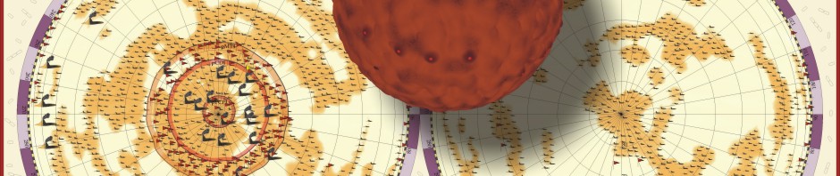
In the case of Escherichia coli such a genomic square is composed of 779 fragments of DNA with an edge length of 1948 micrometers, in the case of our own DNA the genomic square is composed of 35777 fragments with an edge length of 89442 micrometers (this won’t work on my computer). As demonstrated in the following figures, the genomic square still overlaps Escherichia coli cells, but packaging of the material does not seem to be a major problem.

E. coli genome

E.coli and its genome

E. coli genome

E. coli and its genome (front view)

So packaging seems doable, but how is it really done. Here, I will only present one recurring motif of DNA-packaging, which is the use of fractal loops (or helices, or coils). These are exemplified below with molecules 8.500 base pairs long.

The helical conformation of the DNA double helix already shortens the molecules considerably (with the calculations above referring to such double helical molecules, however).

DNA double helix

DNA double helix

Double helices can be arranged into loops.

looped DNA

looped DNA

And these, again, into super-loops, which, of course, is not the last level of looping.

super-looped DNA

super-looped DNA

Nota bene: This is only a concept, the reality is much more complex.

Anyway, these pictures should give an idea, how very long molecules fit into very small spaces.

There is only one geometric mystery remaining (at least to me), connected to the replication of DNA. Replication occurs within the nucleus, so the bulk of DNA has to stay packaged while small segments are unpacked to become replicated. In the end the newly formed molecules are condensed even further (forming chromosomes), to allow the spatial separation of the two copies. How is it possible that the newly formed molecules are not hopelessly knotted? Does anybody have an idea?

Further reading:

Histones: DNA packaging and much more

Scientists unwrap DNA packaging to gain insight into cells

DNA Chromosome packaging animation

A cellular secret to long life

Posted in Genes and Genomes | Tagged , , | Leave a comment